| CPC B63B 79/20 (2020.01) [G06N 3/04 (2013.01)] | 3 Claims |

|
1. A method for forecasting a demand load of a hybrid electric ship by means of working condition classification, comprising the following steps:
Step I. obtaining demand loads bi, at time instants i=1, 2, 3, . . . , for a fixed navigation route of the hybrid electric ship, with a sampling period of one sampling time interval, and with n denoting a number of samples of the demand loads collected from historical navigation data;
Step II. for the time instant i, calculating the following four characteristic parameters: average power ratio
 maximum power ratio Max Pri=max(bi−1, bi−2, bi−3, bi−4, bi−5), minimum power ratio Min Pri=min(bi−1, bi−2, bi−3, bi−4, bi−5) and variance of power ratio
 Step III. establishing a classification model for working conditions, employing a radial basis function as a kernel function of an LS-SVM algorithm: taking xi=[Avg Pri, Max Pri, Min Pri, Pr Vari] as input xi, and taking working condition type of the hybrid electric ship as output yi, to obtain the following constrained optimization equation for a classification plane for working conditions:
 wherein w denoting a weight coefficient vector, γ denoting a penalty coefficient representing a tolerance to a misclassified sample, ei denoting an error at an ith sample point, φ(x) denoting a kernel function, b denoting an offset, and yi denoting a working condition type; solving the above constrained optimization equation by Lagrange multiplier method to obtain:
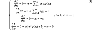
 wherein ai being a Lagrange multiplier corresponding to the i sample; taking partial derivatives of the Lagrange function L(w, b, ei, ai) respective to w, b, ei and ai respectively, and equating the derivatives to 0 according to KKT condition to obtain:
 transforming expression (3) to the following matrix equation:
 wherein y=[y1, y2, . . . , a=[a1, a2, . . . and Ω=yiyjφ(xi)Tφ(xj), i, j=1, 2, 3, . . . ; solving equation (4) to obtain a and b, and obtaining a classification plane as
 Step IV. dividing the demand loads into t intervals equally from 0 to a maximum of the demand loads, regarding each interval as a demand load state, and expressing a demand load state space as E=(E1, E2, E3, . . . , with El=[al1,al2], l=1, 2, 3, . . . , wherein al1 representing a lower bound of an lth state and al2 representing an upper bound of the lth state;
Step V. establishing a Markov prediction model, and constructing a state transition matrix GM of the demand loads to predict a state of a future demand load: denoting the demand load state at a current time instant as El and the demand load state at another time instant as Eo, wherein o=1, 2, 3, . . . ; denoting a number of transition of the demand load state from El to Eo as ml,o, denoting a sum of all the numbers of transition of the demand load state El as mp, and calculating a number of transition from the state El to Eo by means of maximum likelihood estimation:
 to obtain
 wherein the transition of the demand load state from El to Eo implicating that there exists bk and bk+1 such that bk∈El and bk+1∈Eo;
Step VI. constructing a three-layer forward radial basis function neural network, composed of an input layer, a hidden layer and an output layer, and with the demand loads as training output; employing Gaussian function as kernel function of the radial basis function network in the hidden layer; a number v of neurons in the hidden layer is determined by the maximum matrix element method, with the neurons being expressed as:
 wherein, M being an input vector, M=(xx1, xx2, . . . , xxq=[xaq, xbq, xcq], q=1, 2, 3, . . . , xaq representing motor speed, xbq representing set torque, and xcq representing actual torque, with xaq, xbq, and xcq being obtained from the historical navigation data as training input; σl being a width of an lth hidden layer Gaussian function, cl=(cl1, cl2, . . . being a center vector of the lth Gaussian function in the hidden layer, Rl being an output of an lth neuron in the hidden layer;
employing genetic algorithm to obtain optimal parameters of the neural network: firstly, constructing each individual by means of binary coding to consist of the center vector cl, the width σl and a connection weight between the hidden layer and the output layer wls, with a population size T being equal to the number of samples of the demand loads from historical navigation data; initiating the T individuals with random values, and setting a current number of iterations Titeration=0; then performing selection, crossover and mutation; selecting each individual by employing a roulette algorithm, with probability of each individual e being selected and passed on to a next generation as:
 with fitness value for fe being defined as:
 wherein ze denoting a value in the output layer in the current network corresponding to the individual e and de denoting the load demand be;
employing a single-point crossover operator for crossover operation, conducting selection operation by means of optionally selecting two individuals to be crossed over, and setting a crossover probability Pc=0.8; performing simple mutation, that is, performing bit inversion on a binary code of the individual generated subsequent to the crossover operation with a mutation probability Pm, thereby generating a new individual, wherein Pm being set to 0.008; increasing the current number of iterations by one; continuing iteration of crossover operation, selection operation, and simple mutation, until one of stop conditions in the following expression (9) is reached:
 wherein Tmax being a maximum iteration number, and
 being a threshold of positive value;
obtaining an optimal neural network with the center value cl, the width σl, and the connection weight between the hidden layer and the output layer wls upon termination of the iteration;
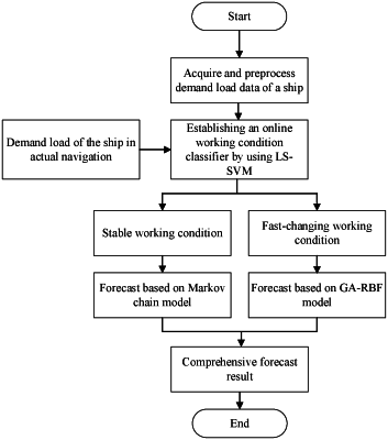
Step VII. for a time instant i in actual navigation, calculating the four characteristic parameters obtained according to the load value at the instants i−1, i−2, i−3, i−4, i−5; inputting the four characteristic parameters into the classification plane d(xi,j) to obtain the working condition type as either a fast-changing working condition or a stable working condition; for the stable working condition, proceeding to Step VIII, and for the fast-changing working condition, proceeding to Step IX;
Step VIII. for the time instant i, obtaining the demand load state Ek1 from Step IV, such that bi∈Ek1;
obtaining k2, such that a number on row k1 and column k2 of the state transition matrix GM is not less than any other number on row k1 of the state transition matrix GM; denoting Ek2 as [al1,al2], then taking the mid-point in [al1,al2] as a predicted demand load for the time instant i+1;
obtaining k3, such that a number on row k2 and column k3 of the state transition matrix GM is not less than any other number on row k2 of the state transition matrix GM; denoting Ek3 as [al3, al4], then taking the mid-point in [al3, al4] as a predicted demand load for the time instant i+2;
obtaining k4, such that a number on row k3 and column k4 of the state transition matrix GM is not less than any other number on row k3 of the state transition matrix GM; denoting Ek4 as [al5,al6], then taking the mid-point in [al5,al6] as a predicted demand load for the time instant i+3;
navigating the ship at the time instants i+1, i+2, and i+3 according to the respective demand loads;
proceeding to Step VII;
Step IX. employing the optimal neural network in Step VI with the connection weight wls to obtain predicted demand loads in 3 time instants subsequent to i as:
 navigating the ship at the time instants i+1, i+2, and i+3 according to the respective demand loads;
proceeding to Step VII.
|