| CPC G06F 30/17 (2020.01) | 1 Claim |

|
1. A reliability-based topology optimization design method for a part structure considering bounded hybrid uncertainties, comprising:
step 1) considering following uncertainties in manufacture and service processes of the part structure: regarding an amplitude and a direction of an external load with insufficient sample information as interval uncertainties, regarding a material property of the part structure with sufficient sample information as a bounded probabilistic uncertainty, and describing a bounded probabilistic uncertainty parameter as a random variable subject to generalized beta distribution;
step 2) discretizing a design domain of the part structure, comprising:
simplifying a force condition of the part structure into a two-dimensional plane stress state, retaining installation holes and removing structural details to improve calculating efficiency, placing the simplified part structure in a regular rectangular design domain, dividing the rectangular design domain into Nx×Ny square elements, where Nx and Ny are numbers of divisions along x, y axes, respectively; and imparting, based on a solid isotropic material with penalization (SIMP) topology optimization framework, each element with a unique design variable ρe∈[0,1] (e=1,2, . . . , Nx·Ny);
step 3) imposing physical constraints and geometric constraints on the discretized structure, comprising:
step 3.1) imposing the physical constraints including fixing or supporting and an external load according to a classical finite element method, which comprises setting the zero displacement at nodes with a constrained degree of freedom, and specifying the node where an external load is applied; and
step 3.2) the geometric constraints including specified holes in the structure and areas where materials are forcibly retained, setting design variables corresponding to elements in the holes as ρhd e≡0, setting design variables corresponding to elements in the areas where the materials are forcibly retained as ρe≡1, and keeping values of the design variables corresponding to elements in the holes and the areas where the materials are to be retained unchanged in subsequent optimization process;
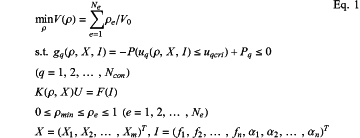
step 4) establishing, by taking a space utilization rate of the design domain as an objective function and taking displacements of several key points of the part structure under a joint influence of interval and bounded probabilistic hybrid uncertainties as reliability constraint performance, a reliability-based topology optimization design model for the part structure, as shown in Eq.1:
 where in Eq. 1, ρ=(ρ1, ρ2, . . . , ρNx·Ny)T is a design vector composed of design variables ρe(e=1,2, . . . , Nx·Ny), and ρmin is a minimum allowable value for the design variables; a total number of elements is Ne=Nx·Ny; a bounded probabilistic uncertainty vector X=(X1, X2, . . . , Xm)T comprises m uncertain material properties of the part structure; an interval uncertainty vector I=(f1, f2, . . . , fn, α1, α2, . . . , αn)T comprises amplitudes f1, f2, . . . , fn and direction angles α1, α2, . . . , αn of n uncertain external loads on the part structure;
where V(ρ) is the space utilization rate of the design domain, corresponding to a total material usage of the part structure, and V0 is a volume of the design domain; where gq(ρ,X,I) is a qth constraint function; uq(ρ,X,I) is a displacement at a qth key point regarded as a qth constraint performance5, denoted as uq for short, and uqcri is an allowable maximum value of uq(ρ, X, I); P(⋅) calculates an occurrence probability of an event in a bracket, Pq is a reliability index of the qth constraint performance, and Ncon is a number of constraint functions; and
where in an equilibrium equation K(ρ,X)U=F(I) of the part structure, K(ρ,X) is a (2(Nx+1)(Ny+1))×(2(Nx+1)(Ny+1))-dimensional global stiffness matrix, which is affected by the design vector ρ and the bounded probabilistic uncertainty vector X; F(I) is a (2(Nx+1)(Ny+1))-dimensional nodal force vector affected by the interval uncertainty vector I; U is a (2(Nx+1)(Ny+1))-dimensional nodal displacement vector; and uq is extracted from U according to uq=LqTU, wherein in a (2(Nx+1)(Ny+1))-dimensional column vector Lq, the element at a position corresponding to the qth key point is 1, and other elements are all 0;
step 5) calculating reliability of a constraint performance under bounded hybrid uncertainties, comprising:
step 5.1) searching a worst working condition of constraint performance uq, comprising:
step 5.1.1) setting X=μX=(μX1, μX2, . . . , μXm) , where μX1, μX2, . . . , μXm are means of uncertainties X1, X2, . . . , Xm, the constraint performance uq is only affected by the interval uncertainty vector; and an uncertain external load Fs(s=1,2, . . . , n) is rewritten as its components in horizontal and vertical directions such as Fs=[fs cos αs, fs sin αs]T;
step 5.1.2) calculating, based on a linear elastic hypothesis in small deformation, displacement Us caused by Fs according to Eq.2 based on esx=[1 0]T, esy=[0 1]T and Fs, where esx and esy are respectively element nodal forces in the horizontal and vertical directions at an point where Fs exerts;
Us=Usx+Usy=usxfs cos αs+usyfs sin αs=[usx,usy]·Fs Eq.2
where usx=[usx 0]T and usy=[0 usy]T are respectively nodal displacement vectors calculated through the equilibrium equation of the part structure when only the element nodal force esx or esy acts;
step 5.1.3) calculating gradients of the constraint performance uq with respect to an amplitude and a direction of an uncertain external load according to Eq.3 and Eq.4:
 step 5.1.4) solving, by utilizing results of Eq.3 and Eq.4, a worst working condition Ĩq by a gradient search algorithm, and an external load of the worst working condition being F=Fq;
step 5.2) restoring μX to X under the worst working condition Ĩq, so that constraint performance ũq=uq(ρ,X,Ĩq) under the worst working condition is only manifested as a probabilistic type, and solving a performance fluctuation under the worst working condition to evaluate reliability, comprising:
step 5.2.1) calculating, according to Eq.5, a gradient of the constraint performance ũq with respect to a bounded probabilistic uncertainty parameter Xi(i=1 2, . . . , m) under the worst working condition:
 where a summation symbol is a combination operation of the element stiffness matrix defined by a finite element theory, ke is an element stiffness matrix, a nodal displacement vector Ũ under the worst working condition is obtained by solving a governing equation KŨ=Fq under the worst working condition; and p is a penalty factor;
step 5.2.2) searching, based on a result of Eq.5, two bounded probabilistic uncertainty vectors minimizing or maximizing uq (ρ,X,Ĩq) respectively according to Eq.6:
 where corresponding to XqL and XqR, global stiffness matrix K is KqL and KqR, respectively, KqL is denoted as KqL=K(ρ,XqL) and KqR is denoted as KqR=K(ρ,XqR), KqL and KqR are uniformly marked as Kq*(*=L,R), the nodal displacement vector Ũ is ŨqL and ŨqR, respectively, and ŨqL and ŨqR are uniformly marked as Ũq*(*=L,R); and
step 5.2.3) denoting ũqL=uq(ρ, XqL, Ĩq) and ũqR=uq(ρ, XqR, Ĩq), defining [ũqL, ũqR] as a performance fluctuation of the constraint performance uq under the worst working condition, and calculating a reliability Rq of the constraint performance according to Eq .7:
 where uqC=(ũqR+ũqL)/2 is a midpoint of the performance fluctuation under the worst working condition; P is a multiplier calculated by P=1(uqW−εu), where εu is a small constant for adjusting reliability at a boundary position of the performance fluctuation under the worst working condition; uqW=(ũqR−ũqL)/2 is a radius of the performance fluctuation under the worst working condition; and γ∈{2i|i∈N+} is a regulatory factor; and
establishing the constraint functions in Eq.1 as Eq.8:
gq(ρ,X,I)=−Rq+Pq≤0(q=1, 2, . . . , Ncon) Eq.8
step 6) calculating gradients of objective and constraint functions with respect to the design variables:
step 6.1) calculating the gradient of the objective function through Eq.9:
 step 6.2) solving the gradient of a constraint function as follows:
step 6.2.1) writing a gradient expression of gq(ρ,X,I) according to a chain rule, as shown in Eq.10:
 step 6.2.2) denoting a function in a bracket of tanh(⋅) in Eq.7 as R(uqcri), and calculating gradient terms ∂gq(ρ,X,I)/∂ũqL and ∂gq(ρ,X,I)/∂ũqR in Eq.10 according to Eq.11:
 where a gradient term ∂R(uqcri)/∂ũq* is as follows:
 step 6.2.3) giving gradient terms ∂ũqL/∂ρe in Eq.10 in a uniform form according to the SIMP framework:
 where Kq* and Ũq*(*=L,P) are defined in 5.2.2; and a gradient term ∂Kq*/∂ρe is calculated according to Eq.15:
 where keq* is an element stiffness matrix extracted from Kq*, and
 keq* keq* is a square matrix reconstructed by performing a combined operation on elements in keq* according to the element stiffness matrix, and is consistent with Kq* in dimensionality; and is a square matrix reconstructed by performing a combined operation on elements in keq* according to the element stiffness matrix, and is consistent with Kq* in dimensionality; andstep 6.2.4) substituting all the gradient terms in Eq.11 to Eq.15 into Eq.10 to obtain a gradient of the constraint function gq(ρ,X,I); and
step 7) updating the design variables by using a moving asymptote algorithm based on the gradients of the objective and constraint functions with respect to the design variables, checking a difference value between an objective function value in a current iteration and an objective function value in a previous iteration, wherein the difference value for a first iteration is defined as an objective function value, and when the difference value is less than a convergence threshold, outputting the updated design variables, or otherwise, repeating the steps 5) to 7).
|