| CPC G01N 27/9006 (2013.01) [G01N 1/44 (2013.01); G01N 25/72 (2013.01); G01N 27/90 (2013.01); G01N 27/9046 (2013.01)] | 1 Claim |
|
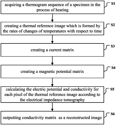
1. A method for eddy current thermography defect reconstruction based on electrical impedance tomography, comprising:
(1): powering on a coil, and then using the coil to excite a specimen under test (hereinafter referred to as specimen), then an induced eddy current will be generated in the specimen, meanwhile, in the process of heating, using an infrared camera to acquire a thermogram sequence of the specimen, which is denoted by thermogram sequence S, where each frame of image of thermogram sequence S is m*n;
(2): for each location of thermogram sequence S, putting pixels there according to time to fit a temperature-time curve, then choosing a slope of a second point of the temperature-time curve as a rate of change of temperature with respect to time, which is denoted by
 where Tij is the pixel value at the second point, row i and column j represent its location, t is the time at the second point, then creating a thermal reference image by taking
 as a pixel, where i=1, 2, . . . , m, j=1, 2, . . . , n;
(3): creating a current matrix by:
3.1) calculating a current amplitude for each pixel of the thermal reference image according to the following heat conduction equation:
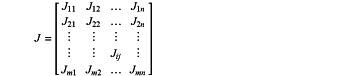
 where Jij is a current amplitude of row i and column j, i=1, 2, . . . , m, j=1, 2, . . . , n, σ* is a conductivity of the specimen, ρ is a density of the specimen, C is a specific heat capacity of the specimen;
3.2): creating a current matrix J:
 (4): creating a magnetic potential matrix by:
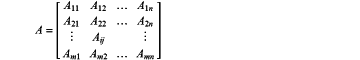
4.1): calculating a magnetic potential for each pixel of the thermal reference image according to the following equation:
 where I is a current in the coil, μ0 is a permeability of air, C is a closed path along the coil, dl is a vector length element along the coil, Rij is a distance from the coil to the pixel of row i and column j of the specimen;
4.2): creating a magnetic potential matrix A:
 (5): calculating the electric potential and conductivity for each pixel of the thermal reference image according to the electrical impedance tomography by:
5.1): inputting initial conductivity matrix σ1, angular frequency ω and iteration termination criteria ε, and initializing iteration number k=1;
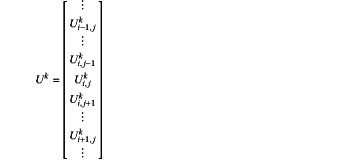
5.2): for iteration k, calculating an electric potential matrix Ûk by traversing all pixels of the thermal reference image, where the electric potential Uki,j of row i and column j satisfies the following equation:
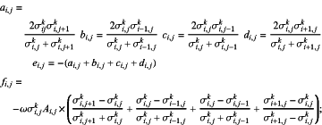
ai,jUki,j+1+bi,jUki−1,j+ci,jUki,j−1+di,jUki+1,j+ei,jUki,j=fi,j
where parameters ai,j, bi,j, ci,j, di,j, ei,j, fi,j satisfy the following equation:
 then creating the following matrix form:
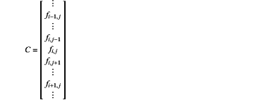
G·Uk=C
where Uk is a electric potential vector, which is created by choosing electric potentials Uki,j from left to right and top to bottom, and putting them from top to bottom:
 where parameter matrix G is composed of parameters ai,j, bi,j, ci,j, di,j, ei,j:
 where vector C is composed of parameter fi,j:
 then calculating electric potential vector Uk according to the following equation:
Uk=G−1·C
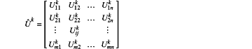
then choosing the electric potentials of electric potential vector Uk from top to bottom, and putting them from left to right and top to bottom to create electric potential matrix Ûk:
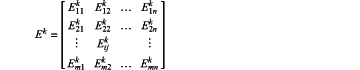
 5.3): calculating electric field intensity matrix Ek of the kth iteration, where electric field intensity Eki,j of row i and column j satisfies the following equation:
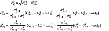 where electric field intensity matrix Ek is:
 5.4): calculating the conductivity matrix σk+1 after the kth iteration, where conductivity matrix σk+1 is:
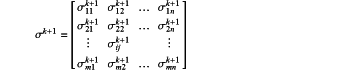 where conductivity σk+1ij of row i and column j is:
 5.5): judging whether the infinite norm ∥σk+1−σk∥∞ is less than iteration termination criteria ε, if not, then adding 1 to iteration number k and returning to step 5.2) to continue iterating, otherwise, going to step (6);
(6): outputting conductivity matrix σk+1, and taking it as a reconstructed image, then taking the low conductivity area of the reconstructed image as the defect profile.
|